Get a Half-life!: Student Worksheet

Name: ___________________________________

A decay function is one in which the values decrease by a constant factor, but it is not linear! These functions are often used to model the decay of a radioactive element. The half-life of a substance is the time it takes to reduce its initial effectiveness by one-half.

Students work in pairs.

Each pair needs:

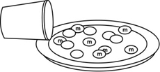
• 1 cup of m&m's
  
• 1 paper plate or box
  
• 1 graphing calculator

1. Collect the Data
   1. Pour m&m's out and count your beginning sample size (N). This will be your N value when T = 0. Enter this value in the table below and put the m&m's back in the cup.
   2. Shake the cup gently and pour the m&m's out in the box or on the paper plate.
   3. Remove all the m&m's with an "m" showing. (You may eat these m&m's only!)
   4. Count the remaining m&m's and enter this value of N into your table next to T = 1.
   5. Put the remaining m&m's back in the cup.
   6. Repeat this process until there are no longer any m&m's with the letter "m" when you empty your cup.
   
   

   Trial Number (T)	0	1	2	3	4	5	6	7
   # of remaining m&m’s (N)

   
   
2. Use the Calculator
   1. Clear out the calculator:
      Press [2nd][Y=]. Enter [4]. Press [ENTER]. This turns off all plots.
      Press [Y=], [CLEAR], down arrow and [CLEAR] until all equations are cleared.
      Press [STAT], [ENTER] to view tables. To clear Lists, press up arrow to highlight L1, press [CLEAR], [ENTER]. Use arrow keys to highlight any other lists and clear.
   2. Enter the data from the table above:
      Press [STAT], choose EDIT by pressing [ENTER] and enter values of T in L1 using down arrow keys and [ENTER].
      Use right arrow key to move over to L2 and enter the values of N in L2.
   3. Graph the Data
      Press [STAT PLOT] ([2nd][Y=]), choose 1 by pressing [ENTER].
      Highlight: ON
      

      Broken line graph
      Xlist: L1
      Ylist: L2
      Mark: first one

      Press [ZOOM], then [9] to set up appropriate window and see graph.
   4. Have the calculator determine the best equation for the data.
      Linear:
      Press [STAT]. Choose CALC[5].
      Type in L1, L2 (press [2nd][1][,][2nd][2] then [ENTER]). You will see y = ax + b and values for a, b, and r.
      Press [Y=], set cursor next to Y1=, press [VARS][5], arrow over to EQ, press [7], the [GRAPH].
      
      Quadratic:
      Press [STAT], choose CALC [6], then type in L1, L2 (like above) and press [ENTER].
      Press [Y=]. Set your cursor next to Y2=.
      Press [VARS][5], arrow over to EQ, press [7], the [GRAPH]. (Adjust the window here to see more of this graph)
      
      Exponential:
      Press [STAT] and choose CALC . Choose A by using the down arrow key until you see "A ExpReg". Press [ENTER].
      Type in L1, L2 as before and then [ENTER]. You will see y = a*b^x (y = abx) and values for a, b, and r.
      Press [Y=] and set your cursor next to Y3=.
      Press [VARS], choose [5], arrow over to EQ, press [7], then [GRAPH].
   
   
3. Analyze the Data
   1. Which graph most clearly approximates a "curve of best fit" for your data?
   2. Why is this called a "half-life"?
   3. What is a good estimate for the length of a "half-life" of m&m's based on your research?

As a result of this activity, students learn to model a real-life situation by collecting data from a few trials, graphing the data, and then drawing a curve of best fit. The student must decide which of the equations best fits his/her data. Sometimes when a student gathers his/her own data, the graph does not make a perfect line or curve.

1. Describe the factors that influenced you to choose your "curve of best fit".
2. Explain how each of the three types of equations, linear, quadratic, and exponential, are different.